In 1924 de Broglie proposed that every moving particle has a wavelength, and within three years electrons had been diffracted by a crystal. This unit computes the wavelengths of electrons, neutrons, atoms, molecules, and a tennis ball, explains the Davisson-Germer experiment and the double slit, shows how single electrons build up an interference pattern dot by dot, and states what happens when the path of a particle is recorded. It ends with interfering molecules of 10,000 atomic mass units and the electron microscope.
Sample unit: the complete text
Unit 2 ended with light behaving as a stream of particles, each carrying a momentum \(p = h/\lambda\). In 1924 a doctoral student in Paris turned this sentence around and proposed that every particle with momentum \(p\) is accompanied by a wave of wavelength \(h/p\). Within three years the wave had been seen in the laboratory, and within sixty years electrons were filmed building up an interference pattern one at a time. This unit follows that path from the hypothesis to the experiments, works out the wavelengths of electrons, neutrons, atoms, molecules, and a tennis ball, and ends with the two places where matter waves are used every day, the electron microscope and the molecule interferometer.
1 De Broglie’s hypothesis
Louis de Broglie (1892-1987) started from a symmetry. Light had been known to be a wave for a century, and Unit 2 showed that it also comes in photons with energy \(E = hf\) and momentum \(p = h/\lambda\). If a wave can carry the properties of a particle, de Broglie asked, why should a particle not carry the properties of a wave? He proposed that the same two relations connect the momentum and energy of any moving body, an electron as much as a photon, to a wavelength and a frequency. The de Broglie wavelength of a particle is the wavelength that goes with its momentum.
The second form follows from the first by solving \(K = \tfrac12 mv^2 = p^2/2m\) for \(p\). An electron that has been accelerated through a voltage \(V\) has gained the kinetic energy \(K = eV\), so its wavelength is \(h/\sqrt{2m_e eV}\), and with the constants put in this is \(1.226\unit{nm}\) divided by the square root of the voltage in volts. A third form is useful for atoms and neutrons in a gas at temperature \(T\), whose mean kinetic energy is \(\tfrac32 k_{\mathrm{B}}T\) with Boltzmann’s constant \(k_{\mathrm{B}}\) (Unit 1). Putting this energy in for \(K\) gives their typical wavelength, \(\lambda = h/\sqrt{3mk_{\mathrm{B}}T}\).
Table 1 collects these numbers with a few more. Two patterns run through the table. The first is that heavier particles at the same speed have shorter wavelengths, because the momentum grows with the mass. The second is that the wavelength falls only with the square root of the kinetic energy, so a thousandfold increase in energy shortens it by a factor of about 32, the square root of 1,000. For everything we can hold in a hand the wavelength is unmeasurably small, and for electrons, neutrons, and atoms it is about the size of an atom. Diffraction, the spreading and interference of a wave at an obstacle, is only noticeable when the obstacle is not much larger than the wavelength, so the wave nature of matter can only show itself at the scale of atoms.
Particle
Kinetic Energy or Speed
Wavelength
Electron
\(54\unit{eV}\)
\(0.167\unit{nm}\)
Electron
\(300\unit{keV}\) (electron microscope)
\(1.97\unit{pm}\)
Neutron
thermal, \(300\unit{K}\)
\(0.145\unit{nm}\)
Helium atom
thermal, \(300\unit{K}\)
\(72.9\unit{pm}\)
Fullerene \(\mathrm{C}_{60}\), \(720\unit{u}\)
\(200\unit{m\,s^{-1}}\)
\(2.77\unit{pm}\)
Tennis ball, \(57\unit{g}\)
\(50\unit{m\,s^{-1}}\)
\(2.3\times10^{-34}\unit{m}\)
Table 1. De Broglie wavelengths of particles from the electron to a tennis ball. The thermal values use the mean kinetic energy \(\tfrac32 k_{\mathrm{B}}T\); the value for the \(300\unit{keV}\) electron includes the relativistic correction of Section 6. The mass unit u is the atomic mass unit, one twelfth of the mass of a carbon-12 atom, and \(1\unit{pm}\) (picometre) is \(10^{-12}\unit{m}\).
2 Electron diffraction
A wave shows itself by diffraction and interference, and for a wavelength of a tenth of a nanometre the only gratings with a fine enough spacing are crystals, in which the atoms sit in rows about \(0.2\) to \(0.4\unit{nm}\) apart. Clinton Davisson (1881-1958) at the Western Electric laboratories in New York, which became the Bell Telephone Laboratories in 1925, had been firing slow electrons at nickel targets since 1921 to study how electrons bounce off metals, and in October 1924 Lester Germer (1896-1971) joined him in this work. In April 1925 a bottle of liquid air exploded next to their apparatus, air entered the vacuum tube, and the hot nickel target oxidized. The long heating needed to clean it turned the fine-grained metal into a few large crystals, because at high temperature the small crystal grains of a metal grow into larger ones. The scattering pattern changed completely, and from then on they worked with a single crystal cut to expose one flat face. In the summer of 1926 Davisson learned on a visit to England that theorists expected electrons to diffract, and in January 1927 the two found what they were looking for.
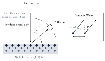
Figure 1. The Davisson-Germer experiment. A beam of electrons falls at right angles on to the face of a nickel crystal, and a collector that moves along an arc measures how many electrons leave in each direction. The rows of atoms in the surface, a distance \(d\) apart, act as a diffraction grating; the inset shows that waves scattered by two neighbouring rows into the direction \(\theta\) differ in path length by \(d\sin\theta\).
Figure 1 shows the arrangement. Electrons of a chosen energy hit the crystal face at right angles, and the collector counts those that leave elastically, with their full energy, as a function of the angle \(\theta\) from the incident direction. Along the surface the atoms form rows with a spacing \(d\), and each row scatters a little of the incoming wave. In a direction \(\theta\), the waves from two neighbouring rows have travelled paths that differ by \(d\sin\theta\), as the inset shows. When this difference is a whole number of wavelengths, the waves from all rows arrive in step and reinforce one another; in other directions they cancel. This is the same condition as for a ruled grating in optics.
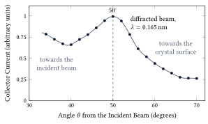
Figure 2. The measurement of 1927. The collector current for \(54\unit{V}\) electrons, read from Figure 10 of Davisson and Germer’s paper in the Physical Review of December 1927, against the angle from the incident beam. The sharp maximum at \(50^\circ\) is the diffracted beam, and it disappears when the voltage is changed by a few volts in either direction. The current scale is the paper’s arbitrary one.
Figure 2 shows their measurement. The beam at \(50^\circ\) appears only when the voltage is near \(54\unit{V}\). At lower voltages the wavelength is longer and the beam moves to larger angles, and at higher voltages it moves toward the incident direction, exactly as the diffraction condition demands. Davisson and Germer went on to find twenty more such beams at different voltages and from different sets of rows, and nineteen of these could be compared with \(\lambda = h/p\). The agreement was within the accuracy of the measurements. Their preliminary report appeared in the journal Nature in April 1927 and the full paper in December of the same year.
Two months after the Nature letter, George Paget Thomson (1892-1975) in Aberdeen reported the same effect in a completely different form. He sent fast electrons, accelerated through tens of thousands of volts, through a thin film of celluloid and later through films of metal, and on a photographic plate behind the film he found rings around the central spot. The films consist of countless tiny crystals in every orientation, so the diffracted beams leave at the same angle \(\theta\) but in every direction around the beam axis, and form cones instead of single spots, exactly as X-rays do when they pass through a powder of small crystals. The radii of the rings gave the wavelength, and it agreed with de Broglie’s formula. Davisson and Thomson shared the Nobel Prize in Physics 1937. Thomson’s father, J. J. Thomson, had received the prize of 1906 for his work on the conduction of electricity through gases, the work in which he had identified the electron as a particle, so the father was honoured for showing that the electron is a particle and the son for showing that it is a wave.
Matter waves were soon found for heavier particles. In 1930 Immanuel Estermann (1900-1973) and Otto Stern (1888-1969) in Hamburg diffracted beams of helium atoms and hydrogen molecules from the surface of a lithium fluoride crystal, and from 1936 on, slow neutrons were diffracted by crystals as well. The technique of Davisson and Germer lives on as low-energy electron diffraction, the method shown on the title page of this unit, which is used today to determine how atoms are arranged in the outermost layer of a surface. Electrons of \(94\unit{V}\), as in that picture, have a wavelength of \(0.126\unit{nm}\).
3 The double slit, one electron at a time
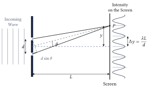
Diffraction by a crystal proved that electrons have a wavelength, but the experiment that shows what this means most clearly is older and simpler. In the first years of the nineteenth century Thomas Young (1773-1829) let light fall on two narrow slits close together and found bright and dark bands on a screen behind them. Figure 3 shows the geometry. The slits are a distance \(d\) apart, the screen is a distance \(L\) behind them, and a point \(P\) on the screen lies a height \(y\) above the axis. Light reaches \(P\) from both slits, and the two waves have travelled paths of different lengths.
Figure 3. The double slit. Waves from the two slits, a distance \(d\) apart, reach the point \(P\) on a screen at distance \(L\) along paths that differ in length by \(d\sin\theta\). Where this difference is a whole number of wavelengths the waves reinforce one another and the screen is bright; the bright bands are \(\Delta y = \lambda L/d\) apart. The curve on the right is the intensity on the screen for the drawn spacing.
For visible light with \(d\) of a fraction of a millimetre and \(L\) of a few metres, the fringes are millimetres apart and easy to see. For electrons of a few tens of kilovolts, the energies used in electron microscopes, the wavelength is about \(5\unit{pm}\), a hundred thousand times smaller than that of visible light, and the slits must be a hundred thousand times finer to give the same fringes. The first person to make such slits was Claus Jönsson (1930-2024) in Tübingen. In 1961 he cut slits a fraction of a micrometre wide and about a micrometre apart into a copper foil, sent \(50\unit{kV}\) electrons through them, magnified the pattern with electron lenses, and photographed fringes exactly like Young’s.
Jönsson’s photographs were taken with a dense beam, so one could still imagine that the electrons somehow interfere with one another. The decisive step was to send the electrons one at a time. Pier Giorgio Merli (1943-2008), Gian Franco Missiroli, and Giulio Pozzi did this in Bologna in 1974 and published it in 1976, and Akira Tonomura (1945-2012) and his colleagues at the Hitachi laboratory in Tokyo repeated it in 1989 with a detector that registered every single electron. Both groups used an electron biprism instead of two slits. A biprism is a wire thinner than a micrometre, held at a small positive voltage between two earthed plates. The electron wave that passes on the left of the wire is bent slightly to the right, the part that passes on the right is bent to the left, and behind the wire the two halves overlap at a small angle, which we call \(2\beta\). Two waves that cross at a small angle \(2\beta\) produce fringes \(\lambda/2\beta\) apart. This is the double-slit formula in disguise, because seen from the screen the two slits are separated by the small angle \(d/L\), and \(\Delta y = \lambda L/d\) is the wavelength divided by that angle, so the biprism formula is the double-slit formula with \(2\beta\) in place of \(d/L\). A biprism is an equivalent double slit, with the advantage that the two beams come from one wide opening and are easy to keep in step.
Figure 4. Tonomura’s experiment of 1989: the detector screen after 11, 200, 6,000, 40,000, and 140,000 electrons (frames a to e). Every bright dot is one electron. The first frames look random, and the fringes emerge only when the dots are counted in thousands. Credit: Akira Tonomura and Hitachi, via Wikimedia Commons, CC BY-SA 3.0; the five frames of the original file are shown side by side.
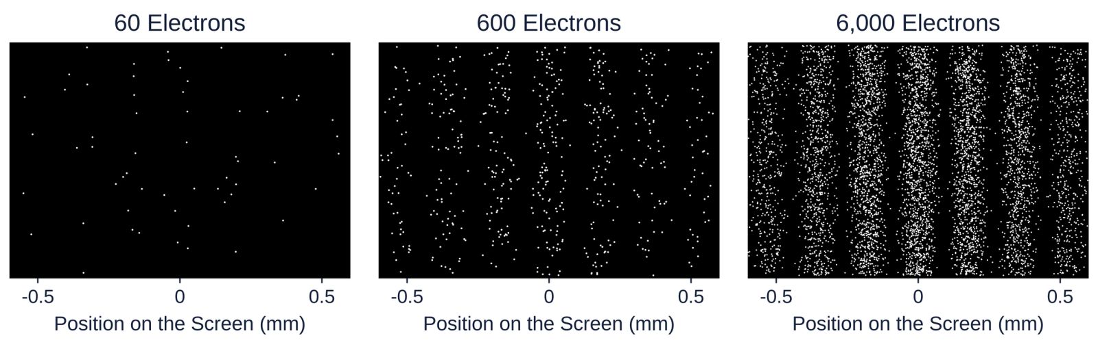
Figure 4 shows what the detector recorded. Each electron arrives as one dot at one place, and nothing about the first dozen dots suggests a wave. The source delivered fewer than a thousand electrons per second, and at \(41\) per cent of the speed of light, which is about \(120{,}000\unit{km}\) travelled every second, that is an average distance of more than \(100\unit{km}\) between one electron and the next, in an apparatus \(1.5\unit{m}\) long. There was never more than one electron in the microscope, so no electron could have interfered with another. Yet after twenty minutes the dots had drawn the fringes of the double slit. The wave that governs where an electron lands belongs to each electron on its own. Paul Dirac (1902-1984) put it in one sentence in his textbook of 1930, where he wrote that each photon interferes only with itself, and the same is true of electrons.
Figure 5. The build-up computed for a double slit of this unit’s own geometry: electrons of \(600\unit{eV}\) (\(\lambda = 50\unit{pm}\)), slits \(50\unit{nm}\) wide and \(280\unit{nm}\) apart, and a screen \(1.0\unit{m}\) behind them, which gives a fringe spacing of \(0.18\unit{mm}\). Each dot is one arrival drawn at random from the double-slit intensity; the height of a dot carries no information. The panels show 60, 600, and 6,000 electrons.
The lesson of these pictures is the central lesson of quantum mechanics, and Unit 4 turns it into mathematics. The wave says how likely the electron is to be found at each place, and it says nothing about where the electron is before it arrives or what shape it has. Where the two waves from the slits reinforce one another, many electrons arrive; where they cancel, none do; and which of the allowed places a particular electron chooses is not determined by anything we can measure beforehand. The square of the wave amplitude is a probability, a rule that Max Born (1882-1970) formulated in 1926 and that carries his name.
For a long time the only double slits for single electrons were biprisms. In 2013 Roger Bach and his colleagues at the University of Nebraska cut two real slits, each \(50\unit{nm}\) wide and \(280\unit{nm}\) apart, into a thin sheet (a membrane) of silicon nitride and sent \(600\unit{eV}\) electrons through them one at a time, which is the geometry of Figure 5. A movable mask allowed them to close either slit. With one slit open the detector showed the broad pattern of a single slit; with both open, the fringes; and the fringes were not the sum of the two single-slit patterns. This is the thought experiment with which Richard Feynman (1918-1988) opened the quantum mechanics volume of his lectures on physics, published in 1965, performed exactly as he described it half a century later.
4 Which-path information and complementarity
Since each electron arrives at one point, it is natural to ask which slit it came through. Suppose we place a detector at each slit that registers an electron passing without stopping it. Then every electron is found at one slit or the other, never at both, and the pattern on the screen changes. The fringes disappear, and what remains is the broad single-slit pattern, the same one that appears when the slits are opened one after the other. The effect does not depend on how strongly the detector disturbs the electron. It has been confirmed in experiments in which the path was recorded without any measurable push on the particle; in 1998 the group of Gerhard Rempe in Konstanz stored the path of each atom in an atom interferometer (a double slit for atoms) in the internal state of the atom itself, that is, in which of two energy levels the atom was left, and the fringes vanished all the same.
Niels Bohr (1885-1962) introduced the word complementarity in a lecture at Como in September 1927. Wave behaviour and particle behaviour, he argued, are both needed to describe an electron, and the experimental arrangements that show one exclude the arrangements that show the other. The statement is also quantitative, because a partial record of the path gives partial fringes. In 1996 Berthold-Georg Englert proved that the fringe contrast \(V\) (1 for fringes with fully dark gaps between them, 0 for no fringes at all) and the distinguishability \(D\) of the two paths (0 when nothing tells them apart, 1 when the record is certain) always obey \(V^2 + D^2 \le 1\), so full path knowledge, \(D = 1\), forces \(V = 0\). The record need not be read by anyone. It is enough that the information exists in the state of some physical system, because the fringes come from adding the two waves, and two waves that are tied to different states of a detector no longer add. Unit 6 shows the other side of the same coin, namely that any device that locates the electron at one slit gives it a momentum kick large enough to wash out the fringes, a connection that Bohr used against Einstein’s objections at the Solvay conference of 1927 (Unit 8).
5 Interference of large molecules
Complementarity raises a practical question. A large molecule is a hot, vibrating, rotating object that constantly interacts with its surroundings, so one might expect that something always records its path and that interference stops at some size. Experiments in Vienna have pushed that limit further and further out. In 1999 Markus Arndt, Anton Zeilinger, and their colleagues sent fullerene molecules, \(\mathrm{C}_{60}\), sixty carbon atoms arranged like the seams of a football, through a diffraction grating. The molecules came from an oven at about \(900\) to \(1{,}000\unit{K}\), flew at a most probable speed (the speed shared by the largest number of molecules in the beam) of \(220\unit{m\,s^{-1}}\), and had a wavelength of \(2.5\unit{pm}\), about 400 times smaller than the molecule itself. The grating, a silicon nitride membrane with slits \(50\unit{nm}\) wide and a period of \(100\unit{nm}\) (the distance from one slit to the next), stood \(1.25\unit{m}\) in front of a detector that ionized the molecules with a laser beam and counted them. The pattern had the diffraction orders exactly where the de Broglie wavelength put them.
The Vienna group then moved to a three-grating interferometer, in which a first grating prepares the wave, a laser standing wave (a laser beam reflected back on itself, whose bright and dark stripes act on the molecules like the bars of a grating) acts as the second grating, and a third grating scans the fringes, and they designed molecules for the purpose. In 2013 they showed interference of molecules of more than \(10{,}000\unit{u}\), each made of 810 atoms, and in 2019 of molecules of more than \(25{,}000\unit{u}\) with about 2,000 atoms, whose de Broglie wavelength was as short as \(53\unit{fm}\) (\(1\unit{fm} = 10^{-15}\unit{m}\)). The molecules are hot, but as long as they emit no photon that could reveal the path, and collide with no gas atom on the way, nothing records which slit they took and the fringes appear. When the gas pressure is raised or the molecules are heated until they radiate, the fringes fade in exactly the way the record of the path predicts. This loss of interference through unwanted records in the surroundings is called decoherence, and Unit 8 returns to it.
Neutrons deserve a paragraph of their own, because they are the particle with which matter waves have been tested most precisely. A neutron is heavy and uncharged, and in a reactor beam it has a wavelength near \(0.1\unit{nm}\). In 1974 Helmut Rauch, Wolfgang Treimer, and Ulrich Bonse in Vienna cut an interferometer from a single perfect crystal of silicon, and since then neutron waves have been split and recombined along paths several centimetres apart. In 1975 such an interferometer showed that the Earth’s gravity shifts the phase of a neutron wave by the amount that quantum mechanics predicts for a particle of the neutron’s mass. In 1988 Zeilinger and his colleagues sent cold neutrons of about \(2\unit{nm}\) wavelength through a double slit roughly a tenth of a millimetre wide and recorded a fringe pattern that agrees with the double-slit formula in every detail.
6 The electron microscope
A microscope cannot show details much smaller than the wavelength of the waves it uses, because a wave bends around any obstacle smaller than itself and carries no sharp image of it. For a light microscope the limit, worked out by Ernst Abbe (1840-1905) in 1873, is about half the wavelength, which for green light of \(550\unit{nm}\) is roughly \(200\unit{nm}\), about a thousand atoms side by side. Matter waves remove this limit, because electrons accelerated through a hundred kilovolts have wavelengths of a few picometres, a hundred times smaller than an atom.
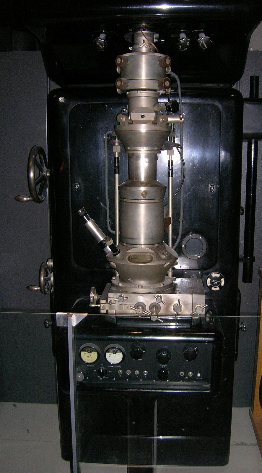
Figure 6. A replica, made in 1980, of the electron microscope with which Ernst Ruska (1906-1988) first surpassed the resolution of the light microscope in Berlin in 1933, on display in the Deutsches Museum in Munich. The column in the middle holds the magnetic lenses; the sample sits between them, and the image is viewed on a fluorescent screen at the bottom. Credit: J Brew, Wikimedia Commons, CC BY-SA 2.0.
At voltages of a hundred kilovolts and more the electrons are fast enough that the simple relation \(K = p^2/2m\) no longer holds. The exact relation between momentum and kinetic energy, \((pc)^2 = K^2 + 2Km_ec^2\), where \(m_ec^2 = 0.511\unit{MeV}\) is the rest energy of the electron (the energy equivalent of its mass), is given here as a fact from the theory of relativity and leads to
\[
\lambda = \frac{h}{p} = \frac{hc}{\sqrt{K^2 + 2Km_ec^2}},
\]
which returns to the de Broglie relation of Section 1 when \(K \ll m_ec^2\).
Ernst Ruska and Max Knoll (1897-1969) built the first electron microscope in Berlin in 1931, and in 1933 Ruska’s instrument resolved finer detail than any light microscope could (Figure 6). Ruska received the Nobel Prize in Physics 1986 for it, more than fifty years later. The irony is that Ruska did not design his microscope as a wave instrument. He thought of electrons as particles steered by magnetic lenses, and when he learned of de Broglie’s waves after the first instrument was built, he was relieved to find that their wavelength was small enough not to spoil the images. Today the same instrument carries the biprism of Tonomura’s experiment, maps the arrangement of atoms in a crystal or a virus, and in its diffraction mode repeats the experiment of Davisson and Germer every day in materials laboratories around the world.
This is one of 16 units
Participants also get the quiz, the further reading, and the final exam.