 Image: Jan Ainali, Wikimedia Commons, CC BY 3.0
How MRI uses quantum mechanics
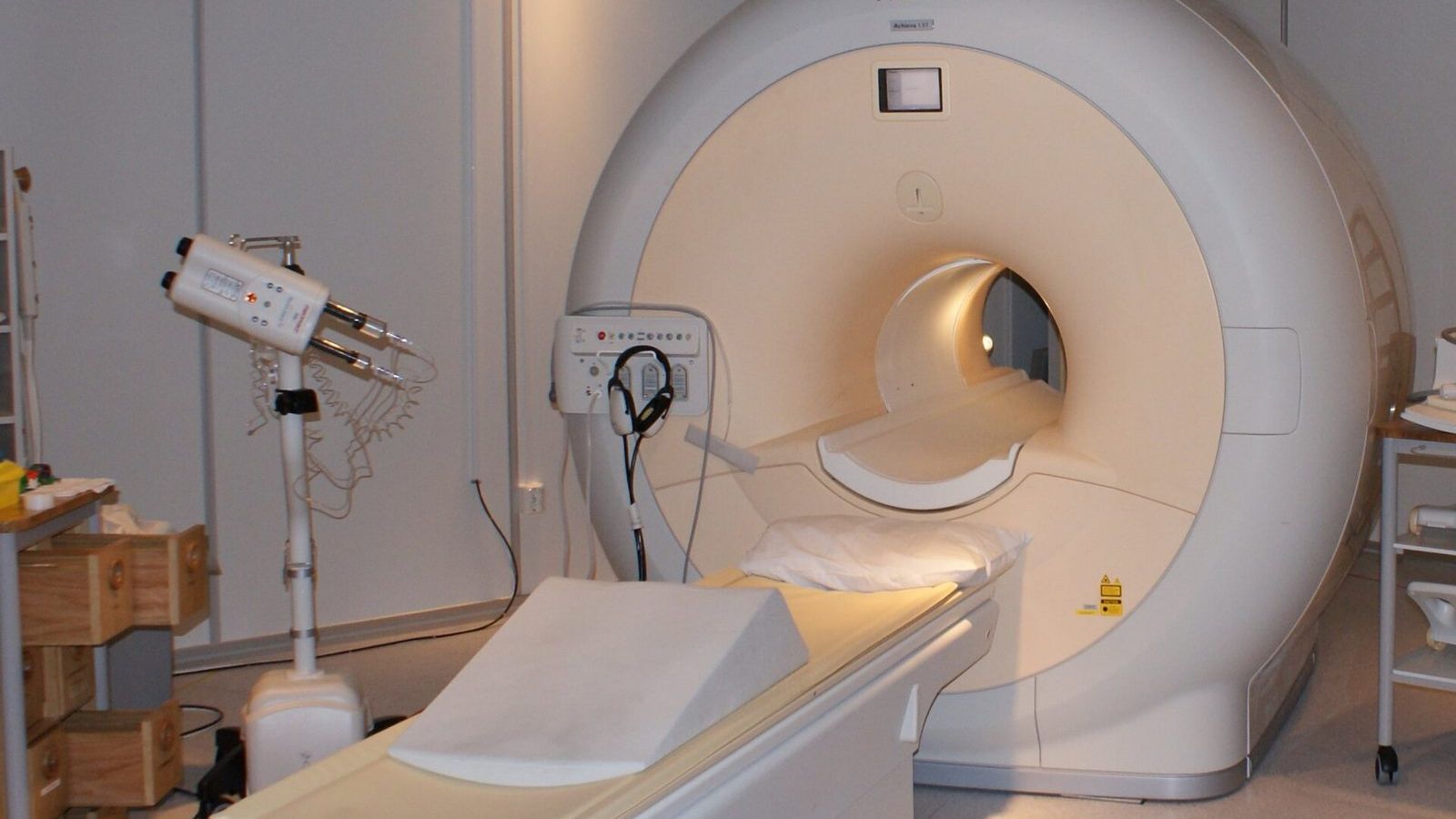
About 60 percent of the human body is water, and every water molecule contains two hydrogen nuclei, which are single protons. Each proton is a spin-1/2 particle with a magnetic moment. In the three tesla field of a modern MRI scanner, a field sixty thousand times stronger than the Earth's, the proton's magnetic moment can take exactly two orientations, with the field or against it, separated in energy by about half a millionth of an electron volt. Everything an MRI scanner does follows from that tiny energy gap.
Two levels and a frequency
A photon with energy equal to the gap between the two proton states has a frequency of
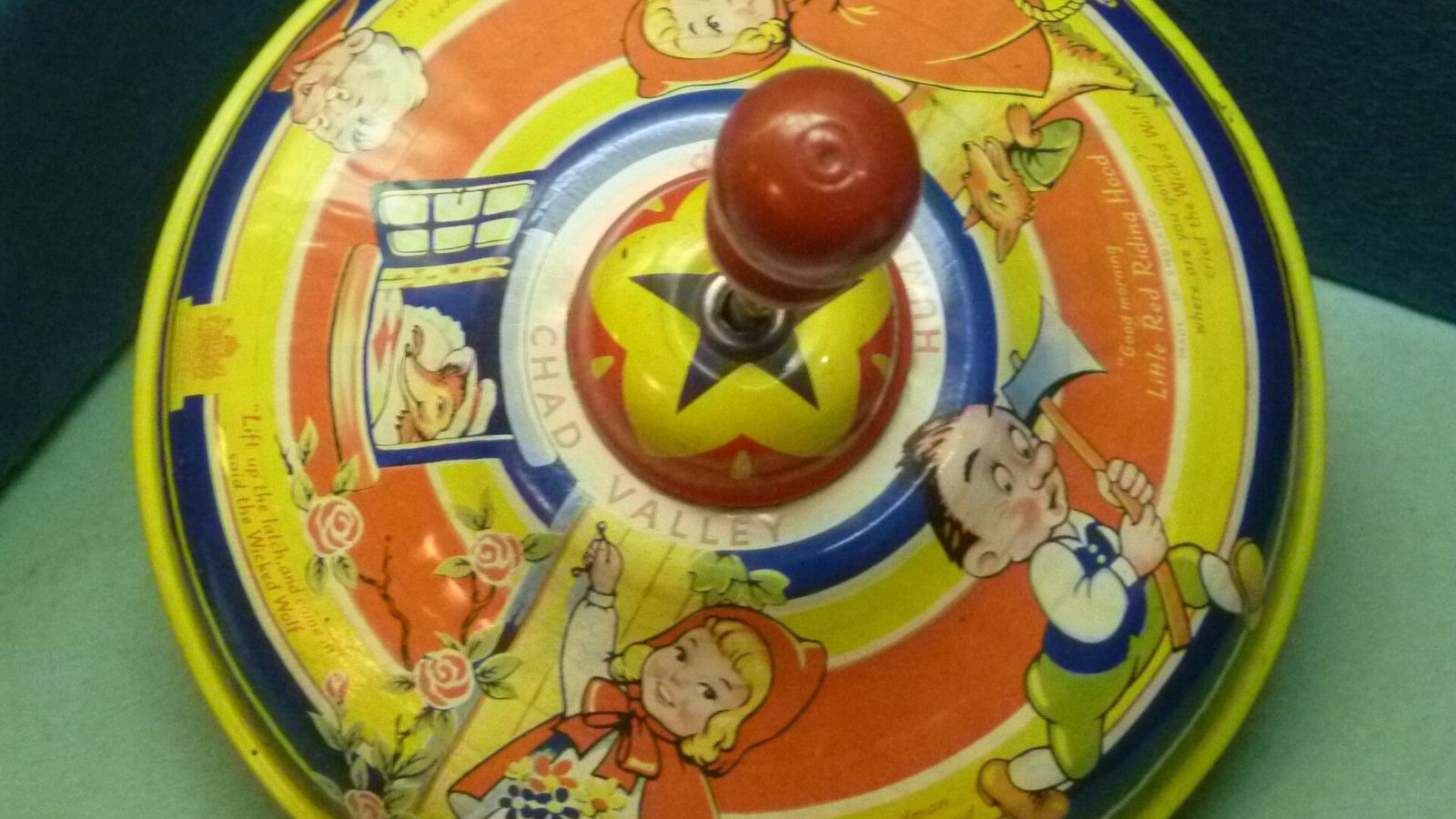
\[ f = \gamma B = 42.58 \text{ MHz per tesla} \times B, \]where \(\gamma\) is the gyromagnetic ratio of the proton, known to ten significant figures. In a 1.5 tesla scanner this is 64 MHz, in a 3 tesla scanner 128 MHz, in the FM radio band. A proton in the lower state can absorb a radio photon at exactly this frequency and flip to the upper state, and nothing happens at any other frequency. This is resonance, and the R in MRI stands for it. The same frequency is the rate at which a proton's magnetic moment, if tilted away from the field, precesses around it, like a spinning top around the vertical. Joseph Larmor worked out the classical version in 1897, and the frequency bears his name.
Why the signal is weak
At body temperature the thermal energy, \(k_B T\), is about 27 millielectron volts, fifty thousand times larger than the gap between the two proton states. The protons are therefore almost equally divided between the two levels. The excess in the lower level, which is all that produces a net magnetization, is about ten protons in a million at 3 tesla. The scanner's whole signal comes from that excess.
This is why the magnet is so strong. The excess grows in proportion to the field, and so does the energy of each radio photon, so the signal grows roughly as the square of the field. A 3 tesla scanner gives four times the signal of a 1.5 tesla one, and research scanners at 7 tesla and above exist for the same reason. The magnet is superconducting, cooled with liquid helium to 4 kelvin, and once the current is started it runs for years without a power supply. Switching it off in an emergency means boiling away the helium, which is why the quench button is behind a cover.
The pulse and the echo
The scan begins with a pulse of radio waves at the Larmor frequency, lasting a few milliseconds. In the quantum description it drives transitions between the two levels and puts each proton into a superposition of up and down; in the equivalent classical description it tips the net magnetization of the tissue away from the field, by 90 degrees for a standard pulse. The tipped magnetization then precesses at 128 MHz, and a precessing magnet induces a voltage in a nearby coil. The receiving coil picks up this voltage, a signal of microvolts, and that is the raw data of MRI.
The signal does not last. Two things happen to it, on two different time scales, and both are what the images actually show. The individual protons precess at slightly different rates, because each sits in a slightly different local field produced by its neighbours, so they drift out of step and their voltages cancel. The time for this is called \(T_2\), and it ranges from about 40 milliseconds in muscle to several hundred milliseconds in fluid. Separately, the magnetization relaxes back along the field as the protons give their extra energy to the surrounding molecules. This time, \(T_1\), is a few hundred milliseconds in fat and over a second in cerebrospinal fluid.
From a signal to an image
A single coil picks up the signal from the whole body at once. To know where each part comes from, the scanner adds to the main field a small gradient, a field that increases from one side of the body to the other, produced by extra coils. Now the Larmor frequency varies with position, by a few kilohertz across the body, and the received signal is a mixture of frequencies, each one tagging a position. A Fourier transform of the signal sorts the frequencies and gives a projection of the proton density along the gradient direction. Switching the gradients in a sequence of directions and phases and transforming the whole data set gives the image. Paul Lauterbur published this idea in 1973, Peter Mansfield made it fast enough to be practical, and the two shared the Nobel Prize in Physiology or Medicine 2003. The loud knocking during a scan is the gradient coils being switched on and off in the main field, which makes them flex.
The contrast between tissues comes from timing. A sequence that samples the signal early and repeats quickly emphasizes differences in \(T_1\), making fat bright and fluid dark; a sequence that waits longer emphasizes \(T_2\), making fluid bright. A tumour, an inflammation, or a bleed changes the local water content and the relaxation times, and so changes the brightness. A radiologist chooses the sequence to make the suspected difference visible. Contrast agents based on gadolinium, a strongly magnetic ion, shorten \(T_1\) in the tissue they reach and light it up.
What the scanner does not do
MRI uses no ionizing radiation. The radio photons carry half a microelectron volt each, ten million times too little to break a chemical bond, and the only heating is the gentle warming of tissue by the radio pulses, which the scanner limits by regulation. The method was known as nuclear magnetic resonance from its discovery in 1946 by Felix Bloch and Edward Purcell, who shared the Nobel Prize in Physics 1952 for it, and the word nuclear was dropped from the medical name in the 1980s because patients found it alarming. The nucleus in question is the proton of hydrogen, and the only thing nuclear about the measurement is where the spin lives.
Chemists have used the same physics since the 1950s to determine the structure of molecules, because the precise Larmor frequency of each proton depends, at the level of parts per million, on the electrons around it. A proton in a methyl group and a proton in a benzene ring precess at slightly different rates, and an NMR spectrum is a list of those rates.
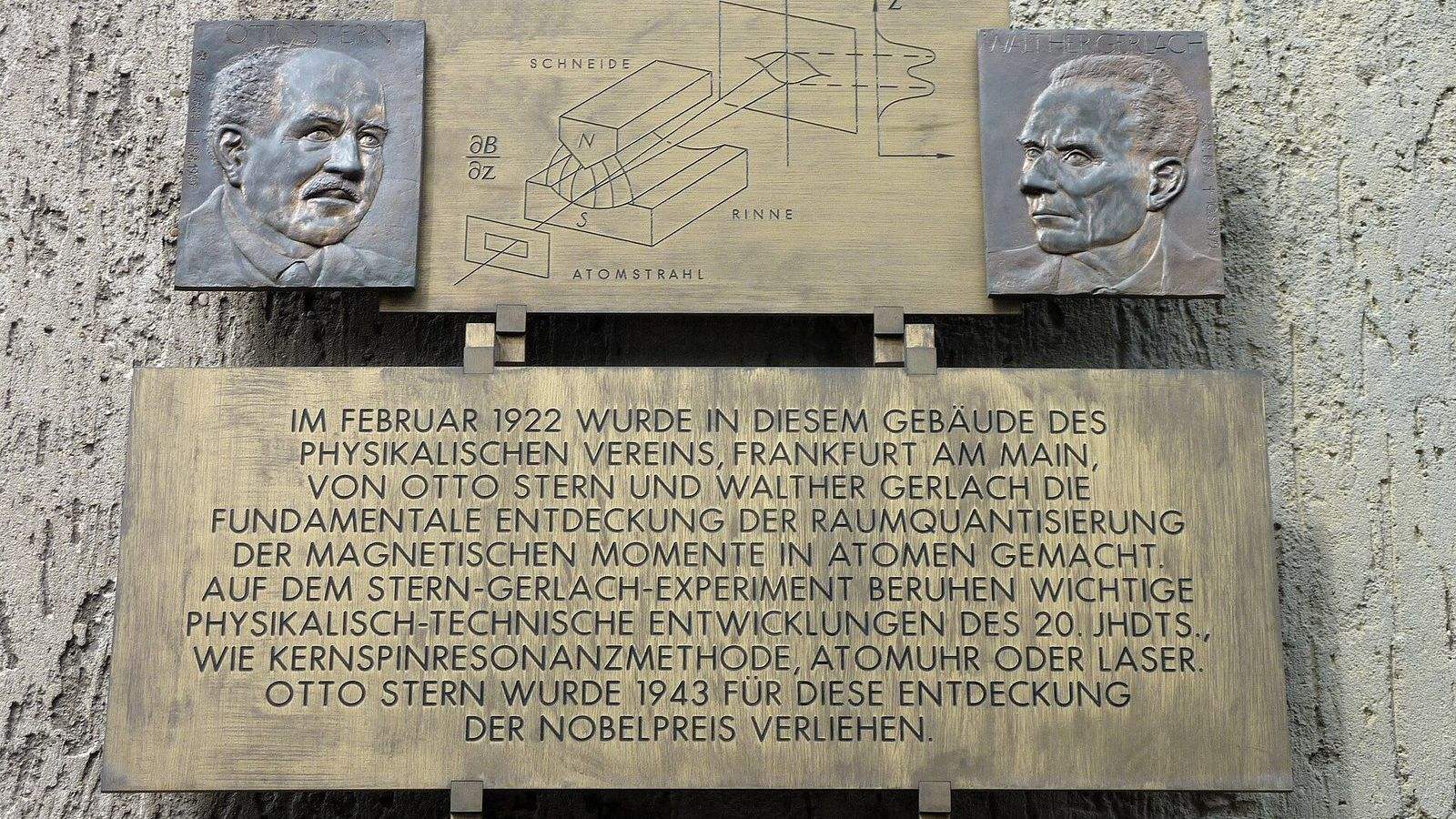
In the Quantum Mechanics Masterclass, spin in a magnetic field is treated in Unit 11, which derives the Larmor frequency, computes the thermal population difference above, and shows how a radio pulse rotates a spin on the Bloch sphere. The two-level system itself is introduced with the Stern-Gerlach experiment earlier in the same unit, and the statistical argument for the ten-in-a-million excess uses the Boltzmann factor first met in Unit 2.